A newer version of the platform is available. Please refresh the page.
Sign Up to Get information about Sales & Events Click Here

A newer version of the platform is available. Please refresh the page.
Reprinted with permission of the Substance Abuse and Mental Health Services Administration www.SAMHSA.gov
U.S. DEPARTMENT OF HEALTH AND HUMAN SERVICES
Substance Abuse and Mental Health Services Administration
Center for Behavioral Health Statistics and Quality
Table of Contents
A. Description of the Survey
A.1 Sample Design
A.2 Data Collection Methodology
A.3 Data Processing
B. Statistical Methods and Measurement
B.1 Target Population
B.2 Sampling Error and Statistical Significance
B.3 Other Information on Data Accuracy
B.4 Measurement Issues
A.1 Sample Design
The sample design for the 2011 National Survey on Drug Use and Health (NSDUH)3 was an extension of a coordinated 5-year design providing estimates for all 50 States plus the District of Columbia initially for the years 2005 through 2009, then continuing through 2011. The respondent universe for NSDUH is the civilian, noninstitutionalized population aged 12 years old or older residing within the United States. The survey covers residents of households (persons living in houses/townhouses, apartments, condominiums; civilians living in housing on military bases, etc.) and persons in noninstitutional group quarters (e.g., shelters, rooming/boarding houses, college dormitories, migratory workers’ camps, halfway houses). Excluded from the survey are persons with no fixed household address (e.g., homeless and/or transient persons not in shelters), active-duty military personnel, and residents of institutional group quarters, such as correctional facilities, nursing homes, mental institutions, and long-term hospitals.
The coordinated design for 2005 through 2009 facilitated a 50 percent overlap in second-stage units (area segments) within each successive 2-year period from 2005 through 2009. The 2010 and 2011 NSDUHs continued the 50 percent overlap by retaining half of the second-stage units from the previous survey. Those segments not retained are considered “retired” from use. Because the coordinated design enabled estimates to be developed by State in all 50 States plus the District of Columbia, States may be viewed as the first level of stratification and as a reporting variable.
In 2011, an oversample was included to help in measuring and reporting on the impact that the April 2010 Deepwater Horizon oil spill had on substance use and mental health along the gulf coast. To that end, the target sample was expanded by 2,000 cases in four Gulf Coast States (Alabama, Florida, Louisiana, and Mississippi), resulting in a total targeted national sample size of 69,500. The 2011 Gulf Coast Oversample (GCO) was attained by supplementing the NSDUH sample with 89 segments in GCO-designated counties and parishes in these four States. These 89 segments were retired from use in the 2009 and 2010 surveys. For more details on the GCO and information about the general 2011 NSDUH sample design, see the 2011 NSDUH sample design report by Morton, Martin, Shook-Sa, Chromy, and Hirsch (2012).
For the 50-State design, 8 States were designated as large sample States (California, Florida, Illinois, Michigan, New York, Ohio, Pennsylvania, and Texas) with pre-oversample target sample sizes of 3,600. In 2011, the actual sample sizes in these States ranged from 3,074 to 4,029.4 For the remaining 42 States and the District of Columbia, the pre-oversample target sample size was 900. Sample sizes in these States ranged from 865 to 1,746 in 2011.5 This approach ensured there was sufficient sample in every State to support State estimation by either direct methods or small area estimation (SAE)6 while at the same time maintaining efficiency for national estimates.
States were first stratified into a total of 900 State sampling regions (SSRs) (48 regions in each large sample State and 12 regions in each small sample State). These regions were contiguous geographic areas designed to yield approximately the same number of interviews.7 Unlike the 1999 through 2001 NHSDAs and the 2002 through 2004 NSDUHs in which the first-stage sampling units were clusters of census blocks called area segments, the first stage of selection for the 2005 through 2011 NSDUHs was census tracts.8 This stage was included to contain sample segments within a single census tract to the extent possible.9
Within each SSR, 48 census tracts were selected with probability proportional to population size. Within sampled census tracts, adjacent census blocks were combined to form the second-stage sampling units or area segments. One area segment was selected within each sampled census tract with probability proportional to population size. Although only 24 segments were needed to support the coordinated 5-year sample, an additional 24 segments were selected to support any supplemental studies that the Substance Abuse and Mental Health Services Administration (SAMHSA) may choose to field. These 24 segments constituted the reserve sample and were available for use in 2010 and 2011. Eight reserve sample segments per SSR were fielded during the 2011 survey year. Four of these segments were retained from the 2010 survey, and four were selected for use in the 2011 survey.
These sampled segments were allocated equally into four separate samples, one for each 3-month period (calendar quarter) during the year. That is, a sample of addresses was selected from two segments10 in each calendar quarter so that the survey was relatively continuous in the field. In each of the area segments, a listing of all addresses was made from which a national sample of 216,521 addresses was selected. Of the selected addresses, 179,293 were determined to be eligible sample units. In these sample units (which can be either households or units within group quarters), sample persons were randomly selected using an automated screening procedure programmed in a handheld computer carried by the interviewers. The number of sample units completing the screening was 156,048. Youths aged 12 to 17 years and young adults aged 18 to 25 years were oversampled at this stage, with 12 to 17 year olds sampled at an actual rate of 87.2 percent and 18 to 25 year olds at a rate of 69.5 percent on average, when they were present in the sampled households or group quarters. Similarly, persons in age groups 26 or older were sampled at rates of 38.2 percent or less, with persons in the eldest age group (50 years or older) sampled at a rate of 8.9 percent on average. The overall population sampling rates were 0.09 percent for 12 to 17 year olds, 0.07 percent for 18 to 25 year olds, 0.02 percent for 26 to 34 year olds, 0.01 percent for 35 to 49 year olds, and 0.01 percent for those 50 or older. Nationwide, 88,536 persons were selected. Consistent with previous surveys in this series, the final respondent sample of 70,109 persons was representative of the U.S. general population (since 1991, the civilian, noninstitutionalized population) aged 12 or older. In addition, State samples were representative of their respective State populations. More detailed information on the disposition of the national screening and interview sample can be found in Appendix B.
A.2 Data Collection Methodology
The data collection method used in NSDUH involves in-person interviews with sample persons, incorporating procedures to increase respondents’ cooperation and willingness to report honestly about their illicit drug use behavior. Confidentiality is stressed in all written and oral communications with potential respondents. Respondents’ names are not collected with the data, and computer-assisted interviewing (CAI) methods are used to provide a private and confidential setting to complete the interview.
Introductory letters are sent to sampled addresses, followed by an interviewer visit. When contacting a dwelling unit (DU), the field interviewer (FI) asks to speak with an adult resident (aged 18 or older) of the household who can serve as the screening respondent. Using a handheld computer, the FI completes a 5-minute procedure with the screening respondent that involves listing all household members along with their basic demographic data. The computer uses the demographic data in a preprogrammed selection algorithm to select zero to two sample persons, depending on the composition of the household. This selection process is designed to provide the necessary sample sizes for the specified population age groupings. In areas where a third or more of the households contain Spanish-speaking residents, the initial introductory letters written in English are mailed with a Spanish version on the back. All interviewers carry copies of this letter in Spanish. If the interviewer is not certified bilingual, he or she will use preprinted Spanish cards to attempt to find someone in the household who speaks English and who can serve as the screening respondent or who can translate for the screening respondent. If no one is available, the interviewer will schedule a time when a Spanish-speaking interviewer can come to the address. In households where a language other than Spanish is encountered, another language card is used to attempt to find someone who speaks English to complete the screening.
The NSDUH interview can be completed in English or Spanish, and both versions have the same content. If the sample person prefers to complete the interview in Spanish, a certified bilingual interviewer is sent to the address to conduct the interview. Because the interview is not translated into any other language, if a sample person does not speak English or Spanish, the interview is not conducted.
Immediately after the completion of the screener, interviewers attempt to conduct the NSDUH interview with each sample person in the household. The interviewer requests the selected respondent to identify a private area in the home to conduct the interview away from other household members. The interview averages about an hour and includes a combination of CAPI (computer-assisted personal interviewing, in which the interviewer reads the questions) and ACASI (audio computer-assisted self-interviewing).
The NSDUH interview consists of core and noncore (i.e., supplemental) sections. A core set of questions critical for basic trend measurement of prevalence estimates remains in the survey every year and comprises the first part of the interview. Noncore questions, or modules, that can be revised, dropped, or added from year to year make up the remainder of the interview. The core consists of initial demographic items (which are interviewer-administered) and self-administered questions pertaining to the use of tobacco, alcohol, marijuana, cocaine, crack cocaine, heroin, hallucinogens, inhalants, pain relievers, tranquilizers, stimulants, and sedatives. Topics in the remaining noncore self-administered sections include (but are not limited to) injection drug use, perceived risks of substance use, substance dependence or abuse, arrests, treatment for substance use problems, pregnancy and health care issues, and mental health issues. Noncore demographic questions (which are interviewer-administered and follow the ACASI questions) address such topics as immigration, current school enrollment, employment and workplace issues, health insurance coverage, and income. In practice, some of the noncore portions of the interview have remained in the survey, relatively unchanged, from year to year (e.g., current health insurance coverage, employment).
Thus, the interview begins in CAPI mode with the FI reading the questions from the computer screen and entering the respondent’s replies into the computer. The interview then transitions to the ACASI mode for the sensitive questions. In this mode, the respondent can read the questions silently on the computer screen and/or listen to the questions read through headphones and enter his or her responses directly into the computer. At the conclusion of the ACASI section, the interview returns to the CAPI mode with the FI completing the questionnaire. Each respondent who completes a full interview is given a $30 cash payment as a token of appreciation for his or her time.
No personal identifying information about the respondent is captured in the CAI record. FIs transmit the completed interview data to RTI in Research Triangle Park, North Carolina, via home telephone analog lines.
After the data are transmitted to RTI, certain cases are selected for verification. The respondents are contacted by RTI to verify the quality of an FI’s work based on information that respondents provide at the end of screening (if no one is selected for an interview at the DU or the entire DU is ineligible for the study) or at the end of the interview. For the screening interview, the adult DU member who served as the screening respondent provides his or her first name and telephone number to the FI, who enters the information into a handheld computer and transmits the data to RTI. For completed interviews, respondents write their home telephone number and mailing address on a quality control form and seal the form in a preaddressed envelope that FIs mail back to RTI. All contact information is kept completely separate from the answers provided during the screening or interview.
Samples of respondents who completed screenings or interviews are randomly selected for verification. These cases are called by telephone interviewers who ask scripted questions designed to determine the accuracy and quality of the data collected. Any cases discovered to have a problem or discrepancy are flagged and routed to a small specialized team of telephone interviewers who recontact respondents for further investigation of the issue(s). Depending on the amount of an FI’s work that cannot be verified through telephone verification, including bad telephone numbers (e.g., incorrect number, disconnected, not in service), a field verification may be conducted. Field verifications involve another FI returning to the sampled DU to verify the accuracy and quality of the data in person. If the verification procedures identify situations in which an FI has falsified data, the FI no longer works on NSDUH. All cases completed that quarter by the FI who falsified data are reworked by the FI conducting the field verification.
A.3 Data Processing
Data that FIs transmit to RTI are processed to create a raw data file in which no logical editing of the data has been done. The raw data file consists of one record for each transmitted interview. Cases are eligible to be treated as final respondents only if they provided data on lifetime use of cigarettes and at least 9 out of 13 of the other substances in the core section of the questionnaire. Written responses to questions (e.g., names of other drugs that were used) are assigned numeric codes as part of the data processing procedures. Even though editing and consistency checks are done by the CAI program during the interview, additional, more complex edits and consistency checks are completed at RTI. Additionally, statistical imputation is used to replace missing or ambiguous values after editing for some key variables. Analysis weights are created so that estimates will be representative of the target population. Details of the editing, imputation, and weighting procedures for 2011 will appear in the 2011 NSDUH Methodological Resource Book, which is in process. Until that volume becomes available, refer to the 2010 NSDUH Methodological Resource Book (RTI International, 2012).
A.3.1 Data Coding and Logical Editing
With the exception of industry and occupation data, coding of written answers that respondents or interviewers typed was performed at RTI for the 2011 NSDUH. These written answers include mentions of drugs that respondents had used or other responses that did not fit a previous response option (subsequently referred to as “OTHER, Specify” data). Coding of the “OTHER, Specify” variables was accomplished through computer-assisted survey procedures and the use of a secure Web site that allowed for coding and review of the data. The computer-assisted procedures entailed a database check for a given “OTHER, Specify” variable that contained typed entries and the associated numeric codes. If an exact match was found between the typed response and an entry in the system, the computer-assisted procedures assigned the appropriate numeric code. Typed responses that did not match an existing entry were coded through the Web-based coding system. Data on the industries in which respondents worked and respondents’ occupations were assigned numeric industry and occupation codes by staff at the U.S. Census Bureau.
As noted above, the CAI program included checks that alerted respondents or interviewers when an entered answer was inconsistent with a previous answer in a given module. In this way, the inconsistency could be resolved while the interview was in progress. However, not every inconsistency was resolved during the interview, and the CAI program did not include checks for every possible inconsistency that might have occurred in the data.
Therefore, the first step in processing the raw NSDUH data was logical editing of the data. Logical editing involved using data from within a respondent’s record to (a) reduce the amount of item nonresponse (i.e., missing data) in interview records, including identification of items that were legitimately skipped; (b) make related data elements consistent with each other; and (c) identify ambiguities or inconsistencies to be resolved through statistical imputation procedures (see Section A.3.2).
For example, if respondents reported that they never used a given drug, the CAI logic skipped them out of all remaining questions about use of that drug. In the editing procedures, the skipped variables were assigned codes to indicate that the respondents were lifetime nonusers. Similarly, respondents were instructed in the prescription psychotherapeutics modules (i.e., pain relievers, tranquilizers, stimulants, and sedatives) not to report the use of over-the-counter (OTC) drugs. Therefore, if a respondent’s only report of lifetime use of a particular type of “prescription” psychotherapeutic drug was for an OTC drug, the respondent was logically inferred never to have been a nonmedical user of the prescription drugs in that psychotherapeutic category.
In addition, respondents could report that they were lifetime users of a drug but not provide specific information on when they last used it. In this situation, a temporary “indefinite” value for the most recent period of use was assigned to the edited recency-of-use variable (e.g., “Used at some point in the lifetime LOGICALLY ASSIGNED”), and a final, specific value was statistically imputed. The editing procedures for key drug use variables also involved identifying inconsistencies between related variables so that these inconsistencies could be resolved through statistical imputation. For example, if a respondent reported last using a drug more than 12 months ago and also reported first using it at his or her current age, both of those responses could not be true. In this example, the inconsistent period of most recent use was replaced with an “indefinite” value, and the inconsistent age at first use was replaced with a missing data code. These indefinite or missing values were subsequently imputed through statistical procedures to yield consistent data for the related measures, as discussed in the next section.
A.3.2 Statistical Imputation
For some key variables that still had missing or ambiguous values after editing, statistical imputation was used to replace these values with appropriate response codes. For example, a response is ambiguous if the editing procedures assigned a respondent’s most recent use of a drug to “Used at some point in the lifetime,” with no definite period within the lifetime. In this case, the imputation procedure assigns a value for when the respondent last used the drug (e.g., in the past 30 days, more than 30 days ago but within the past 12 months, more than 12 months ago). Similarly, if a response is completely missing, the imputation procedures replace missing values with nonmissing ones.
For most variables, missing or ambiguous values are imputed in NSDUH using a methodology called predictive mean neighborhoods (PMN), which was developed specifically for the 1999 survey and has been used in all subsequent survey years. PMN allows for the following: (1) the ability to use covariates to determine donors is greater than that offered in the hot-deck imputation procedure, (2) the relative importance of covariates can be determined by standard modeling techniques, (3) the correlations across response variables can be accounted for by making the imputation multivariate, and (4) sampling weights can be easily incorporated in the models. The PMN method has some similarity with the predictive mean matching method of Rubin (1986) except that, for the donor records, Rubin used the observed variable value (not the predictive mean) to compute the distance function. Also, the well-known method of nearest neighbor imputation is similar to PMN, except that the distance function is in terms of the original predictor variables and often requires somewhat arbitrary scaling of discrete variables. PMN is a combination of a model-assisted imputation methodology and a random nearest neighbor hot-deck procedure. The hot-deck procedure within the PMN method ensures that missing values are imputed to be consistent with nonmissing values for other variables. Whenever feasible, the imputation of variables using PMN is multivariate, in which imputation is accomplished on several response variables at once. Variables imputed using PMN are the core demographic variables, core drug use variables (recency of use, frequency of use, and age at first use), income, health insurance, and noncore demographic variables for work status, immigrant status, and the household roster.
In the modeling stage of PMN, the model chosen depends on the nature of the response variable. In the 2011 NSDUH, the models included binomial logistic regression, multinomial logistic regression, Poisson regression, and ordinary linear regression, where the models incorporated the sampling design weights.
In general, hot-deck imputation replaces an item nonresponse (missing or ambiguous value) with a recorded response that is donated from a “similar” respondent who has nonmissing data. For random nearest neighbor hot-deck imputation, the missing or ambiguous value is replaced by a responding value from a donor randomly selected from a set of potential donors. Potential donors are those defined to be “close” to the unit with the missing or ambiguous value according to a predefined function called a distance metric. In the hot-deck procedure of PMN, the set of candidate donors (the “neighborhood”) consists of respondents with complete data who have a predicted mean close to that of the item nonrespondent. The predicted means are computed both for respondents with and without missing data, which differs from Rubin’s method where predicted means are not computed for the donor respondent (Rubin, 1986). In particular, the neighborhood consists of either the set of the closest 30 respondents or the set of respondents with a predicted mean (or means) within 5 percent of the predicted mean(s) of the item nonrespondent, whichever set is smaller. If no respondents are available who have a predicted mean (or means) within 5 percent of the item nonrespondent, the respondent with the predicted mean(s) closest to that of the item nonrespondent is selected as the donor.
In the univariate case (where only one variable is imputed using PMN), the neighborhood of potential donors is determined by calculating the relative distance between the predicted mean for an item nonrespondent and the predicted mean for each potential donor, then choosing those means defined by the distance metric. The pool of donors is restricted further to satisfy logical constraints whenever necessary (e.g., age at first crack use must not be less than age at first cocaine use).
Whenever possible, missing or ambiguous values for more than one response variable are considered together. In this (multivariate) case, the distance metric is a Mahalanobis distance, which takes into account the correlation between variables (Manly, 1986), rather than a Euclidean distance. The Euclidean distance is the square root of the sum of squared differences between each element of the predictive mean vector for the respondent and the predictive mean vector for the nonrespondent. The Mahalanobis distance standardizes the Euclidean distance by the variance-covariance matrix, which is appropriate for random variables that are correlated or have heterogeneous variances. Whether the imputation is univariate or multivariate, only missing or ambiguous values are replaced, and donors are restricted to be logically consistent with the response variables that are not missing. Furthermore, donors are restricted to satisfy “likeness constraints” whenever possible. That is, donors are required to have the same values for variables highly correlated with the response. For example, donors for the age at first use variable are required to be of the same age as recipients, if at all possible. If no donors are available who meet these conditions, these likeness constraints can be loosened. Further details on the PMN methodology are provided by Singh, Grau, and Folsom (2002).
Although statistical imputation could not proceed separately within each State due to insufficient pools of donors, information about each respondent’s State of residence was incorporated in the modeling and hot-deck steps. For most drugs, respondents were separated into three “State usage” categories as follows: respondents from States with high usage of a given drug were placed in one category, respondents from States with medium usage into another, and the remainder into a third category. This categorical “State rank” variable was used as one set of covariates in the imputation models. In addition, eligible donors for each item nonrespondent were restricted to be of the same State usage category (i.e., the same “State rank”) as the nonrespondent.
In the 2011 NSDUH, the majority of variables that underwent statistical imputation required less than 5 percent of their records to be logically assigned or statistically imputed. Variables for measures that are highly sensitive or that may not be known to younger respondents (e.g., family income) often have higher rates of item nonresponse. In addition, certain variables that are subject to a greater number of skip patterns and consistency checks (e.g., frequency of use in the past 12 months and past 30 days) often require greater amounts of imputation.
A.3.3 Development of Analysis Weights
The general approach to developing and calibrating analysis weights involved developing design-based weights as the product of the inverse of the selection probabilities at each selection stage. Since 2005, NSDUH has used a four-stage sample selection scheme in which an extra selection stage of census tracts was added before the selection of a segment. Thus, the design-based weights,  , incorporate an extra layer of sampling selection to reflect the sample design change. Adjustment factors,
  , then were applied to the design-based weights to adjust for nonresponse, to poststratify to known population control totals, and to control for extreme weights when necessary. In view of the importance of State-level estimates with the 50-State design, it was necessary to control for a much larger number of known population totals. Several other modifications to the general weight adjustment strategy that had been used in past surveys also were implemented for the first time beginning with the 1999 CAI sample.
Weight adjustments were based on a generalization of Deville and Särndal’s (1992) logit model. This generalized exponential model (GEM) (Folsom & Singh, 2000) incorporates unit-specific bounds  for the adjustment factor as follows:
where  are prespecified centering constants, such that
  and
and  . The variables
  are user-specified bounds, and
  is the column vector of p model parameters corresponding to the p covariates x. The -parameters are estimated by solving
where  denotes control totals that could be either nonrandom, as is generally the case with poststratification, or random, as is generally the case for nonresponse adjustment.
The final weights  minimize the distance function
  defined as
This general approach was used at several stages of the weight adjustment process, including (1) adjustment of household weights for nonresponse at the screener level, (2) poststratification of household weights to meet population controls for various household-level demographics by State, (3) adjustment of household weights for extremes, (4) poststratification of selected person weights, (5) adjustment of responding person weights for nonresponse at the questionnaire level, (6) poststratification of responding person weights, and (7) adjustment of responding person weights for extremes.
Every effort was made to include as many relevant State-specific covariates (typically defined by demographic domains within States) as possible in the multivariate models used to calibrate the weights (nonresponse adjustment and poststratification steps). Because further subdivision of State samples by demographic covariates often produced small cell sample sizes, it was not possible to retain all State-specific covariates (even after meaningful collapsing of covariate categories) and still estimate the necessary model parameters with reasonable precision. Therefore, a hierarchical structure was used in grouping States with covariates defined at the national level, at the census division level within the Nation, at the State group within the census division, and, whenever possible, at the State level. In every case, the controls for the total population within a State and the five age groups (12 to 17, 18 to 25, 26 to 34, 35 to 49, 50 or older) within a State were maintained except that, in the last step of poststratification of person weights, six age groups (12 to 17, 18 to 25, 26 to 34, 35 to 49, 50 to 64, 65 or older) were used. Census control totals by age, race, gender, and Hispanic origin were required for the civilian, noninstitutionalized population of each State. Beginning with the 2002 NSDUH, the Population Estimates Branch of the U.S. Census Bureau has produced the necessary population estimates for the same year as each NSDUH survey in response to a special request.
Census control totals for the 2011 NSDUH weights were based on population estimates from the 2010 decennial census, whereas the control totals for the 2010 NSDUH weights still were based on the 2000 census. Section B.4.3 in Appendix B discusses the results of an investigation assessing the effects of using control totals based on the 2010 census instead of the 2000 census for estimating substance use in 2010.
Consistent with the surveys from 1999 onward, control of extreme weights through separate bounds for adjustment factors was incorporated into the GEM calibration processes for both nonresponse and poststratification. This is unlike the traditional method of winsorization in which extreme weights are truncated at prespecified levels and the trimmed portions of weights are distributed to the nontruncated cases. In GEM, it is possible to set bounds around the prespecified levels for extreme weights, then the calibration process provides an objective way of deciding the extent of adjustment (or truncation) within the specified bounds. A step was included to poststratify the household-level weights to obtain census-consistent estimates based on the household rosters from all screened households. An additional step poststratified the selected person sample to conform to the adjusted roster estimates. This additional step takes advantage of the inherent two-phase nature of the NSDUH design. The respondent poststratification step poststratified the respondent person sample to external census data (defined within the State whenever possible, as discussed above).
For certain populations of interest, 2 years of NSDUH data were combined to obtain annual averages. The person-level weights for estimates based on the annual averages were obtained by dividing the analysis weights for the 2 specific years by a factor of 2.
In the 2011 NSDUH, the GCO sample was integrated into the main study sample. The weighting process accounted for the oversampling without additional adjustment needing to be implemented. Special analysis weights were developed for studies focused on the gulf coast area, but these were not used for any estimates for this report.
B.1 Target Population
The estimates of drug use prevalence from the National Survey on Drug Use and Health (NSDUH) are designed to describe the target population of the survey—the civilian, noninstitutionalized population aged 12 or older living in the United States. This population includes almost 98 percent of the total U.S. population aged 12 or older. However, it excludes some small subpopulations that may have very different drug use patterns. For example, the survey excludes active military personnel, who have been shown to have significantly lower rates of illicit drug use. The survey also excludes two groups that have been shown to have higher rates of illicit drug use: persons living in institutional group quarters, such as prisons and residential drug use treatment centers, and homeless persons not living in a shelter. Readers are reminded to consider the exclusion of these subpopulations when interpreting results. Appendix C describes other surveys that provide data for some of these populations.
B.2 Sampling Error and Statistical Significance
This report includes national estimates that were drawn from a set of tables referred to as “detailed tables” that are available at https://www.samhsa.gov/data/. The national estimates, along with the associated standard errors (SEs, which are the square roots of the variances), were computed for all detailed tables using a multiprocedure package, SUDAAN® Software for Statistical Analysis of Correlated Data. This software accounts for the complex survey design of NSDUH in estimating the SEs (RTI International, 2008). The final, nonresponse-adjusted, and poststratified analysis weights were used in SUDAAN to compute unbiased design-based drug use estimates.
The sampling error of an estimate is the error caused by the selection of a sample instead of conducting a census of the population. The sampling error may be reduced by selecting a large sample and/or by using efficient sample design and estimation strategies, such as stratification, optimal allocation, and ratio estimation. The use of probability sampling methods in NSDUH allows estimation of sampling error from the survey data. SEs have been calculated using SUDAAN for all estimates presented in this report using a Taylor series linearization approach that takes into account the effects of NSDUH’s complex design features. The SEs are used to identify unreliable estimates and to test for the statistical significance of differences between estimates.
B.2.1 Variance Estimation for Totals
The variances and SEs of estimates of means and proportions can be calculated reasonably well in SUDAAN using a Taylor series linearization approach. Estimates of means or proportions,  , such as drug use prevalence estimates for a domain d, can be expressed as a ratio estimate:
 , D
, D
where  is a linear statistic estimating the number of substance users in the domain d and
  is a linear statistic estimating the total number of persons in domain d (including both users and nonusers). The SUDAAN software package is used to calculate direct estimates of and (and, therefore,
  ) and also can be used to estimate their respective SEs. A Taylor series approximation method implemented in SUDAAN provides the estimate for the SE of .
When the domain size, , is free of sampling error, an estimate of the SE for the total number of substance users is
 . D
. D
This approach is theoretically correct when the domain size estimates, , are among those forced to match their respective U.S. Census Bureau population estimates through the weight calibration process. In these cases, is not subject to a sampling error induced by the NSDUH design. Section A.3.3 in Appendix A contains further information about the weight calibration process. In addition, more detailed information about the weighting procedures for 2011 will appear in the 2011 NSDUH Methodological Resource Book, which is in process. Until that volume becomes available, refer to the 2010 NSDUH Methodological Resource Book (RTI International, 2012).
For estimated domain totals, , where is not fixed (i.e., where domain size estimates are not forced to match the U.S. Census Bureau population estimates), this formulation still may provide a good approximation if it can be assumed that the sampling variation in is negligible relative to the sampling variation in . This is a reasonable assumption for many cases in this study.
For some subsets of domain estimates, the above approach can yield an underestimate of the SE of the total when was subject to considerable variation. Because of this underestimation, alternatives for estimating SEs of totals were implemented. Since the 2005 NSDUH report, a “mixed” method approach has been implemented for all detailed tables to improve the accuracy of SEs and to better reflect the effects of poststratification on the variance of total estimates. This approach assigns the methods of SE calculation to domains (i.e., subgroups for which the estimates were calculated) within tables so that all estimates among a select set of domains with fixed were calculated using the formula above, and all other estimates were calculated directly in SUDAAN, regardless of what the other estimates are within the same table. The set of domains considered controlled (i.e., those with a fixed ) was restricted to main effects and two-way interactions in order to maintain continuity between years. Domains consisting of three-way interactions may be controlled in a single year but not necessarily in preceding or subsequent years. The use of such SEs did not affect the SE estimates for the corresponding proportions presented in the same sets of tables because all SEs for means and proportions are calculated directly in SUDAAN. As a result of the use of this mixed-method approach, the SEs for the total estimates within many detailed tables were calculated differently from those in NSDUH reports prior to the 2005 report.
Table B.1 at the end of this appendix contains a list of domains with a fixed that were used in the weight calibration process. This table includes both the main effects and two-way interactions and may be used to identify the method of SE calculation employed for estimates of totals. For example, Table 1.23 in the 2011 detailed tables presents estimates of illicit drug use among persons aged 18 or older within the domains of gender, Hispanic origin and race, education, and current employment. Estimates among the total population (age main effect), males and females (age by gender interaction), and Hispanics and non-Hispanics (age by Hispanic origin interaction) were treated as controlled in this table, and the formula above was used to calculate the SEs. The SEs for all other estimates, including white and black or African American (age by Hispanic origin by race interaction) were calculated directly from SUDAAN. Estimates presented in this report for racial groups are for non-Hispanics. Thus, the domain for whites by age group in the weight calibration process in Table B.1 is a two-way interaction. However, published estimates for whites by age group in this report and in the 2011 detailed tables actually represent a three-way interaction: white by Hispanic origin (i.e., not Hispanic) by age group.
B.2.2 Suppression Criteria for Unreliable Estimates
As has been done in past NSDUH reports, direct estimates from NSDUH that are designated as unreliable are not shown in this report and are noted by asterisks (*) in figures containing such estimates. The criteria used to define unreliability of direct estimates from NSDUH are based on the prevalence (for proportion estimates), relative standard error (RSE) (defined as the ratio of the SE over the estimate), nominal (actual) sample size, and effective sample size for each estimate. These suppression criteria for various NSDUH estimates are summarized in Table B.2 at the end of this appendix.
Proportion estimates ( ), or rates, within the range [
 ], and the corresponding estimated numbers of users were suppressed if
or
Using a first-order Taylor series approximation to estimate  and
and  , the following equation was derived and used for computational purposes when applying a suppression rule dependent on effective sample size:
or
 . D
. D
The separate formulas for  produce a symmetric suppression rule; that is, if is suppressed, l − will be suppressed as well (see Figure B.1 following Table B.2). When
  , the symmetric properties of the rule produce a local minimum effective sample size of 50 at = .2 and at = .8. Using the minimum effective sample size for the suppression rule would mean that estimates of between .05 and .95 would be suppressed if their corresponding effective sample sizes were less than 50. Within this same interval, a local maximum effective sample size of 68 is found at = .5. To simplify requirements and maintain a conservative suppression rule, estimates of between .05 and .95 were suppressed if they had an effective sample size below 68.
In addition, a minimum nominal sample size suppression criterion (n = 100) that protects against unreliable estimates caused by small design effects and small nominal sample sizes was employed; Table B.2 shows a formula for calculating design effects. Prevalence estimates also were suppressed if they were close to 0 or 100 percent (i.e., if < .00005 or if ≥ .99995).
Estimates of totals were suppressed if the corresponding prevalence rates were suppressed. Estimates of means that are not bounded between 0 and 1 (e.g., mean of age at first use) were suppressed if the RSEs of the estimates were larger than .5 or if the nominal sample size was smaller than 10 respondents.
B.2.3 Statistical Significance of Differences
This section describes the methods used to compare prevalence estimates in this report. Customarily, the observed difference between estimates is evaluated in terms of its statistical significance. Statistical significance is based on the p value of the test statistic and refers to the probability that a difference as large as that observed would occur because of random variability in the estimates if there were no difference in the prevalence estimates for the population groups being compared. The significance of observed differences in this report is reported at the .05 level. When comparing prevalence estimates, the null hypothesis (no difference between prevalence estimates) was tested against the alternative hypothesis (there is a difference in prevalence estimates) using the standard difference in proportions test expressed as
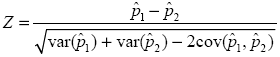 , D
, D
where  = first prevalence estimate,
  = second prevalence estimate,
  = variance of first prevalence estimate,
  = variance of second prevalence estimate, and
  = covariance between and . In cases where significance tests between years were performed, the prevalence estimate from the earlier year becomes the first estimate, and the prevalence estimate from the later year becomes the second estimate (e.g., 2010 is the first estimate and 2011 the second).
Under the null hypothesis, Z is asymptotically distributed as a standard normal random variable. Therefore, calculated values of Z can be referred to the unit normal distribution to determine the corresponding probability level (i.e., p value). Because the covariance term between the two estimates is not necessarily zero, SUDAAN was used to compute estimates of Z along with the associated p values using the analysis weights and accounting for the sample design as described in Appendix A. A similar procedure and formula for Z were used for estimated totals. Whenever it was necessary to calculate the SE outside of SUDAAN (i.e., when domains were forced by the weighting process to match their respective U.S. Census Bureau population estimates), the corresponding test statistics also were computed outside of SUDAAN.
When comparing population subgroups across three or more levels of a categorical variable, log-linear chi-square tests of independence of the subgroups and the prevalence variables were conducted using SUDAAN in order to first control the error level for multiple comparisons. If Shah’s Wald F test (transformed from the standard Wald chi-square) indicated overall significant differences, the significance of each particular pairwise comparison of interest was tested using SUDAAN analytic procedures to properly account for the sample design (RTI International, 2008). Using the published estimates and SEs to perform independent t tests for the difference of proportions usually will provide the same results as tests performed in SUDAAN. However, where the significance level is borderline, results may differ for two reasons: (1) the covariance term is included in SUDAAN tests, whereas it is not included in independent t tests; and (2) the reduced number of significant digits shown in the published estimates may cause rounding errors in the independent t tests.
As part of a comparative analysis discussed in Chapter 8, prevalence estimates from the Monitoring the Future (MTF) study, sponsored by the National Institute on Drug Abuse (NIDA), were presented for recency measures of selected substances (see Tables 8.1 to 8.6). The analyses focused on prevalence estimates for 8th and 10th graders and prevalence estimates for young adults aged 19 to 24 for 2002 through 2011. Estimates for the 8th and 10th grade students were calculated using MTF data as the simple average of the 8th and 10th grade estimates. Estimates for young adults aged 19 to 24 were calculated using MTF data as the simple average of three modal age groups: 19 and 20 years, 21 and 22 years, and 23 and 24 years. Published results were not available from NIDA for significant differences in prevalence estimates between years for these subgroups, so testing was performed using information that was available.
For the 8th and 10th grade average estimates, tests of differences were performed between 2011 and the 9 prior years. Estimates for persons in grade 8 and grade 10 were considered independent, simplifying the calculation of variances for the combined grades. Across years, the estimates for 2011 involved samples independent of those in 2002 to 2009. For 2010 and 2011, however, the sample of schools overlapped 50 percent, creating a covariance in the estimates. Design effects published in Johnston et al. (2012) for adjacent and nonadjacent year testing were used.
For the 19- to 24-year-old age group, tests of differences were done assuming independent samples between years an odd number of years apart because two distinct cohorts a year apart were monitored longitudinally at 2-year intervals. This is appropriate for comparisons of 2002, 2004, 2006, 2008, and 2010 data with 2011 data. However, this assumption results in conservative tests for comparisons of 2003, 2005, 2007, and 2009 data with 2011 data because testing did not take into account covariances associated with repeated observations from the longitudinal samples. Estimates of covariances were not available.
Complete details on testing between NSDUH and MTF can be found in Section B.2.3 in Appendix B of the 2010 national findings report (Center for Behavioral Health Statistics and Quality [CBHSQ], 2011). This discussion also includes variance estimation in the MTF data for testing between adjacent survey years.
B.3 Other Information on Data Accuracy
The accuracy of survey estimates can be affected by nonresponse, coding errors, computer processing errors, errors in the sampling frame, reporting errors, and other errors not due to sampling. These types of “nonsampling errors” and their impact are reduced through data editing, statistical adjustments for nonresponse, close monitoring and periodic retraining of interviewers, and improvement in quality control procedures.
Although these types of errors often can be much larger than sampling errors, measurement of most of these errors is difficult. However, some indication of the effects of some types of these errors can be obtained through proxy measures, such as response rates, and from other research studies.
B.3.1 Screening and Interview Response Rate Patterns
In 2011, respondents continued to receive a $30 incentive in an effort to maximize response rates. The weighted screening response rate (SRR) is defined as the weighted number of successfully screened households11 divided by the weighted number of eligible households (as defined in Table B.3), or
 , D
, D
where  is the inverse of the unconditional probability of selection for the household and excludes all adjustments for nonresponse and poststratification defined in Section A.3.3 of Appendix A. Of the 179,293 eligible households sampled for the 2011 NSDUH, 156,048 were screened successfully, for a weighted screening response rate of 87.0 percent (Table B.3). At the person level, the weighted interview response rate (IRR) is defined as the weighted number of respondents divided by the weighted number of selected persons (see Table B.4), or
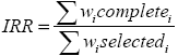 , D
, D
where  is the inverse of the probability of selection for the person and includes household-level nonresponse and poststratification adjustments (adjustments 1, 2, and 3 in Section A.3.3 of Appendix A). To be considered a completed interview, a respondent must provide enough data to pass the usable case rule.12 In the 156,048 screened households, a total of 88,536 sample persons were selected, and completed interviews were obtained from 70,109 of these sample persons, for a weighted IRR of 74.4 percent (Table B.4). A total of 13,311 (18.1 percent) sample persons were classified as refusals or parental refusals, 2,917 (3.4 percent) were not available or never at home, and 2,199 (4.1 percent) did not participate for various other reasons, such as physical or mental incompetence or language barrier (see Table B.4, which also shows the distribution of the selected sample by interview code and age group). Among demographic subgroups, the weighted IRR was higher among 12 to 17 year olds (85.0 percent), females (76.1 percent), blacks (79.8 percent), persons in the South (76.9 percent), and residents of nonmetropolitan areas (77.0 percent) than among other related groups (Table B.5).
The overall weighted response rate, defined as the product of the weighted screening response rate and weighted interview response rate or
 , D
, D
was 64.7 percent in 2011. Nonresponse bias can be expressed as the product of the nonresponse rate ( ) and the difference between the characteristic of interest between respondents and nonrespondents in the population (
 ). By maximizing NSDUH response rates, it is hoped that the bias due to the difference between the estimates from respondents and nonrespondents is minimized. Drug use surveys are particularly vulnerable to nonresponse because of the difficult nature of accessing heavy drug users. However, in a study that matched 1990 census data to 1990 NHSDA nonrespondents,13 it was found that populations with low response rates did not always have high drug use rates. For example, although some populations were found to have low response rates and high drug use rates (e.g., residents of large metropolitan areas and males), other populations had low response rates and low drug use rates (e.g., older adults and high-income populations). Therefore, many of the potential sources of bias tend to cancel each other in estimates of overall prevalence (Gfroerer, Lessler, & Parsley, 1997a).
B.3.2 Inconsistent Responses and Item Nonresponse
Among survey participants, item response rates were generally very high for most drug use items. However, respondents could give inconclusive or inconsistent information about whether they ever used a given drug (i.e., “yes” or “no”) and, if they had used a drug, when they last used it; the latter information is needed to identify those lifetime users of a drug who used it in the past year or past month. In addition, respondents could give inconsistent responses to items such as when they first used a drug compared with their most recent use of a drug. These missing or inconsistent responses first are resolved where possible through a logical editing process. Additionally, missing or inconsistent responses are imputed using statistical methodology. These imputation procedures in NSDUH are based on responses to multiple questions, so that the maximum amount of information is used in determining whether a respondent is classified as a user or nonuser, and if the respondent is classified as a user, whether the respondent is classified as having used in the past year or the past month. For example, ambiguous data on the most recent use of cocaine are statistically imputed based on a respondent’s data for use (or most recent use) of tobacco products, alcohol, inhalants, marijuana, hallucinogens, and nonmedical use of prescription psychotherapeutic drugs. Nevertheless, editing and imputation of missing responses are potential sources of measurement error. For more information on editing and statistical imputation, see Sections A.3.1 and Sections A.3.2 of Appendix A. Details of the editing and imputation procedures for 2011 also will appear in the 2011 NSDUH Methodological Resource Book, which is in process. Until that volume becomes available, refer to the 2010 NSDUH Methodological Resource Book (RTI International, 2012).
B.3.3 Data Reliability
A reliability study was conducted as part of the 2006 NSDUH to assess the reliability of responses to the NSDUH questionnaire. An interview/reinterview method was employed in which 3,136 individuals were interviewed on two occasions during 2006 generally 5 to 15 days apart; the initial interviews in the reliability study were a subset of the main study interviews. The reliability of the responses was assessed by comparing the responses of the first interview with the responses from the reinterview. Responses from the first interview and reinterview that were analyzed for response consistency were raw data that had been only minimally edited for ease of analysis and had not been imputed (see Sections A.3.1 and A.3.2 in this report).
This section summarizes the results for the reliability of selected variables related to substance use and demographic characteristics. Reliability is expressed by estimates of Cohen’s kappa (κ) (Cohen, 1960), which can be interpreted according to benchmarks proposed by Landis and Koch (1977, p. 165): (a) poor agreement for kappas less than 0.00, (b) slight agreement for kappas of 0.00 to 0.20, (c) fair agreement for kappas of 0.21 to 0.40, (d) moderate agreement for kappas of 0.41 to 0.60, (e) substantial agreement for kappas of 0.61 to 0.80, and (f) almost perfect agreement for kappas of 0.81 to 1.00.
The kappa values for the lifetime and past year substance use variables (marijuana use, alcohol use, and cigarette use) all showed almost perfect response consistency, ranging from 0.82 for past year marijuana use to 0.93 for lifetime marijuana use and past year cigarette use. The value obtained for the substance dependence or abuse measure in the past year showed substantial agreement (0.67), while the substance abuse treatment variable showed almost perfect consistency in both the lifetime (0.89) and past year (0.87). The variables for age at first use of marijuana and perceived great risk of smoking marijuana once a month showed substantial agreement (0.74 and 0.68, respectively). The demographic variables showed almost perfect agreement, ranging from 0.95 for current enrollment in school to 1.00 for gender. For further information on the reliability of a wide range of measures contained in NSDUH, see the complete methodology report (Chromy et al., 2010).
B.3.4 Validity of Self-Reported Substance Use
Most substance use prevalence estimates, including those produced for NSDUH, are based on self-reports of use. Although studies generally have supported the validity of self-report data, it is well documented that these data may be biased (underreported or overreported). The bias varies by several factors, including the mode of administration, the setting, the population under investigation, and the type of drug (Aquilino, 1994; Brener et al., 2006; Harrison & Hughes, 1997; Tourangeau & Smith, 1996; Turner, Lessler, & Gfroerer, 1992). NSDUH utilizes widely accepted methodological practices for increasing the accuracy of self-reports, such as encouraging privacy through audio computer-assisted self-interviewing (ACASI) and providing assurances that individual responses will remain confidential. Comparisons using these methods within NSDUH have shown that they reduce reporting bias (Gfroerer, Eyerman, & Chromy, 2002). Various procedures have been used to validate self-report data, such as biological specimens (e.g., urine, hair, saliva), proxy reports (e.g., family member, peer), and repeated measures (e.g., recanting) (Fendrich, Johnson, Sudman, Wislar, & Spiehler, 1999). However, these procedures often are impractical or too costly for general population epidemiological studies (SRNT Subcommittee on Biochemical Verification, 2002).
A study cosponsored by the Substance Abuse and Mental Health Services Administration (SAMHSA) and the National Institute on Drug Abuse (NIDA) examined the validity of NSDUH self-report data on drug use among persons aged 12 to 25. The study found that it is possible to collect urine and hair specimens with a relatively high response rate in a general population survey, and that most youths and young adults reported their recent drug use accurately in self-reports (Harrison, Martin, Enev, & Harrington, 2007). However, there were some reporting differences in either direction, with some respondents not reporting use but testing positive, and some reporting use but testing negative. Technical and statistical problems related to the hair tests precluded presenting comparisons of self-reports and hair test results, while small sample sizes for self-reports and positive urine test results for opiates and stimulants precluded drawing conclusions about the validity of self-reports of these drugs. Further, inexactness in the window of detection for drugs in biological specimens and biological factors affecting the window of detection could account for some inconsistency between self-reports and urine test results.
B.3.5 Revised Estimates for 2006 to 2010
During regular data collection and processing checks for the 2011 NSDUH, data errors were identified. These errors resulted from fraudulent cases submitted by field interviewers and affected the data for Pennsylvania (2006 to 2010) and Maryland (2008 and 2009). Although all fraudulent interview cases were removed from the data files, the affected screening cases were not removed because they were part of the assigned sample. Instead, these screening cases were assigned a final screening code of 39 (“Fraudulent Case”) and treated as incomplete with unknown eligibility. The screening eligibility status for these cases then was imputed. Those cases that were imputed to be eligible were treated as unit nonrespondents for weighting purposes; however, these cases were not treated differently from other unit nonrespondents in the weighting process (see Section A.3.3 in Appendix A). In Table B.3, cases that were imputed to be eligible are classified with a final code of 39 (“Fraudulent Case”). The cases that were imputed to be ineligible did not contribute to the weights and are reported as “Other, Ineligible” in Table B.3. Because all of these cases were treated either as ineligible or as unit nonrespondents at the screening level, they were excluded from the interview data in Table B.4. However, some estimates for 2006 to 2010 in the 2011 national findings report and the 2011 detailed tables, as well as other new reports, may differ from corresponding estimates found in some previous reports or tables.
These errors had minimal impact on the national estimates and no effect on direct estimates for the other 48 States and the District of Columbia. In reports where model-based small area estimation techniques are used, estimates for all States may be affected, even though the errors were concentrated in only two States. In reports that do not use model-based estimates, the only estimates appreciably affected are estimates for Pennsylvania, Maryland, the mid-Atlantic division, and the Northeast region.
The 2011 national findings report and detailed tables do not include State-level or model-based estimates. However, they do include estimates for the mid-Atlantic division and the Northeast region. Single-year estimates based on 2006 to 2010 data and pooled 2008 and 2009 data may differ from previously published estimates. Tables and estimates based only on 2011 data are unaffected by these data errors.
Caution is advised when comparing data from older reports with data from more recent reports that are based on corrected data files. As discussed above, comparisons of estimates for Pennsylvania, Maryland, the mid-Atlantic division, and the Northeast region are of most concern, while comparisons of national data or data for other States and regions are essentially still valid. CBHSQ within SAMHSA is producing a selected set of corrected versions of reports and tables. In particular, CBHSQ has released a set of modified detailed tables that include revised 2006 to 2010 estimates for the mid-Atlantic division and the Northeast region for certain key measures. CBHSQ does not recommend making comparisons between unrevised 2006 to 2010 estimates and estimates based on 2011 data for the geographic areas of greatest concern.
B.4 Measurement Issues
B.4.1 Incidence
In epidemiological studies, incidence is defined as the number of new cases of a disease occurring within a specific period of time. Similarly, in substance use studies, incidence refers to the first use of a particular substance.
In the 2004 NSDUH national findings report (Office of Applied Studies [OAS], 2005), a new measure related to incidence was introduced and since then has become the primary focus of Chapter 5 in this national findings report series. The incidence measure is termed as “past year initiation” and refers to respondents whose date of first use of a substance was within the 12 months prior to their interview date. This measure is determined by self-reported past year use, age at first use, year and month of recent new use, and the interview date.
Since 1999, the survey questionnaire has allowed for collection of year and month of first use for recent initiates (i.e., persons who used a particular substance for the first time in a given survey year). Month, day, and year of birth also are obtained directly or are imputed for item nonrespondents as part of the data postprocessing. Additionally, the computer-assisted interviewing (CAI) instrument records and provides the date of the interview. By imputing a day of first use within the year and month of first use, a specific date of first use,  , can be used for estimation purposes.
Past year initiation among persons using a substance in the past year can be viewed as an indicator variable defined as follows:
 , D
, D
where  ,
,  , and
, and  , denote the day, month, and year of the interview, respectively, and
  denotes the date of first use.
The calculation of this estimate does not take into account whether a respondent initiated substance use while a resident of the United States. This method of calculation has little effect on past year estimates and allows for direct comparability with other standard measures of substance use because the populations of interest for the measures will be the same (i.e., both measures examine all possible respondents and are not restricted to those initiating substance use only in the United States).
One important note for incidence estimates is the relationship between main categories and subcategories of substances (e.g., illicit drugs would be a main category, and inhalants and marijuana would be subcategories in relation to illicit drugs). For most measures of substance use, any member of a subcategory is by necessity a member of the main category (e.g., if a respondent is a past month user of a particular drug, then he or she is also a past month user of illicit drugs in general). However, this is not the case with regard to incidence statistics. Because an individual can only be an initiate of a particular substance category (main or sub) a single time, a respondent with lifetime use of multiple substances may not, by necessity, be included as a past year initiate of a main category, even if he or she were a past year initiate for a particular subcategory because his or her first initiation of other substances within the main category could have occurred earlier.
In addition to estimates of the number of persons initiating use of a substance in the past year, estimates of the mean age of past year initiates of these substances are computed. Unless specified otherwise, estimates of the mean age at initiation in the past 12 months have been restricted to persons aged 12 to 49 so that the mean age estimates reported are not influenced by those few respondents who were past year initiates and were aged 50 or older. As a measure of central tendency, means are influenced heavily by the presence of extreme values in the data, and this constraint should increase the utility of these results to health researchers and analysts by providing a better picture of the substance use initiation behaviors among the civilian, noninstitutionalized population in the United States. This constraint was applied only to estimates of mean age at first use and does not affect estimates of the numbers of new users or the incidence rates.
Although past year initiates aged 26 to 49 are assumed not to be as likely as past year initiates aged 50 or older to influence mean ages at first use, caution still is advised in interpreting trends in these means. For example, the estimate of 49,000 persons aged 26 to 49 who were past year initiates of marijuana in 2009 was significantly different from the estimate of 138,000 past year initiates in this age group in 2011 (Table B.6). However, the estimate of 210,000 past year marijuana initiates aged 26 to 49 in 2010 was not significantly different from the number in 2011. In addition, the mean age at first use of marijuana among past year marijuana initiates aged 26 to 49 was higher in 2010 than in 2011, but the mean ages at first use among past year initiates in this age group were similar between 2011 and other years (Table B.7).
Because NSDUH is a survey of persons aged 12 years old or older at the time of the interview, younger individuals in the sample dwelling units are not eligible for selection into the NSDUH sample. Some of these younger persons may have initiated substance use during the past year. As a result, past year initiate estimates suffer from undercoverage if a reader assumes that these estimates reflect all initial users instead of only for those above the age of 11. For earlier years, data can be obtained retrospectively based on the age at and date of first use. As an example, persons who were 12 years old on the date of their interview in the 2011 survey may report having initiated use of cigarettes between 1 and 2 years ago; these persons would have been past year initiates reported in the 2010 survey had persons who were 11 years old on the date of the 2010 interview been allowed to participate in the survey. Similarly, estimates of past year use by younger persons (age 10 or younger) can be derived from the current survey, but they apply to initiation in prior years and not the survey year.
To get an impression of the potential undercoverage in the current year, reports of substance use initiation reported by persons aged 12 or older were estimated for the years in which these persons would have been 1 to 11 years younger. These estimates do not necessarily reflect behavior by persons 1 to 11 years younger in the current survey. Instead, the data for the 11 year olds reflect initiation in the year prior to the current survey, the data for the 10 year olds reflect behavior between the 12th and 23rd months prior to this year’s survey, and so on. A very rough way to adjust for the difference in the years that the estimate pertains to without considering changes in the population is to apply an adjustment factor to each age-based estimate of past year initiates. This adjustment factor can be based on a ratio of lifetime users aged 12 to 17 in the current survey year to the same estimate for the prior applicable survey year. To illustrate the calculation, consider past year use of alcohol. In the 2011 survey, 75,681 persons 12 years old were estimated to have initiated use of alcohol between 1 and 2 years earlier. These persons would have been past year initiates in the 2010 survey conducted on the same dates had the 2010 survey covered younger persons. The estimated number of lifetime users currently aged 12 to 17 was 8,610,370 for 2011 and 8,621,883 for 2010, indicating fewer overall initiates of alcohol use among persons aged 17 or younger in 2011. Thus, an adjusted estimate of initiation of alcohol use by persons who were 11 years old in 2011 is given by
 . D
. D
This yielded an adjusted estimate of 75,580 persons 11 years old on a 2011 survey date and initiating use of alcohol in the past year:
 . D
. D
A similar procedure was used to adjust the estimated number of past year initiates among persons who would have been 10 years old on the date of the interview in 2009 and for younger persons in earlier years. The overall adjusted estimate for past year initiates of alcohol use by persons 11 years of age or younger on the date of the interview was 163,428, or about 3.5 percent of the estimate based on past year initiation by persons 12 or older only (163,428 ÷ 4,699,084 = 0.0348). Based on similar analyses, the estimated undercoverage of past year initiates was 3.1 percent for cigarettes, 0.7 percent for marijuana, and 17.0 percent for inhalants.
The undercoverage of past year initiates aged 11 or younger also affects the mean age at first use estimate. An adjusted estimate of the mean age at first use was calculated using a weighted estimate of the mean age at first use based on the current survey and the numbers of persons aged 11 or younger in the past year obtained in the aforementioned analysis for estimating undercoverage of past year initiates. Analysis results showed that the mean age at first use was changed from 17.1 to 16.8 for alcohol, from 17.2 to 16.9 for cigarettes, from 17.5 to 17.4 for marijuana, and from 16.4 to 15.1 for inhalants. The decreases reported above are comparable with results generated in prior survey years.
B.4.2 Illicit Drug and Alcohol Dependence and Abuse
The 2011 NSDUH CAI instrumentation included questions that were designed to measure alcohol and illicit drug dependence and abuse. For these substances,14 dependence and abuse questions were based on the criteria in the Diagnostic and Statistical Manual of Mental Disorders, 4th edition (DSM-IV) (American Psychiatric Association [APA], 1994). Specifically, for marijuana, hallucinogens, inhalants, and tranquilizers, a respondent was defined as having dependence if he or she met three or more of the following six dependence criteria:
For alcohol, cocaine, heroin, pain relievers, sedatives, and stimulants, a seventh withdrawal criterion was added. A respondent was defined as having dependence if he or she met three or more of seven dependence criteria. The seventh withdrawal criterion is defined by a respondent reporting having experienced a certain number of withdrawal symptoms that vary by substance (e.g., having trouble sleeping, cramps, hands tremble).
For each illicit drug and alcohol, a respondent was defined as having abused that substance if he or she met one or more of the following four abuse criteria and was determined not to be dependent on the respective substance in the past year:
Criteria used to determine whether a respondent was asked the dependence and abuse questions during the interview included responses from the core substance use questions and the frequency of substance use questions, as well as the noncore substance use questions. Missing or incomplete responses in the core substance use and frequency of substance use questions were imputed. However, the imputation process did not take into account reported data in the noncore (i.e., substance dependence and abuse) CAI modules. Very infrequently, this may result in responses to the dependence and abuse questions that were inconsistent with the imputed substance use or frequency of substance use.
For alcohol and marijuana, respondents were asked the dependence and abuse questions if they reported substance use on more than 5 days in the past year, or if they reported any substance use in the past year but did not report their frequency of past year use. Therefore, inconsistencies could have occurred where the imputed frequency of use response indicated less frequent use than required for respondents to be asked the dependence and abuse questions originally. For alcohol, for example, about 42,000 respondents were past year alcohol users in 2011. Of these, fewer than 100 respondents (about 0.2 percent) were asked the alcohol dependence and abuse questions, but their final imputed frequency of use indicated that they used alcohol on 5 or fewer days in the past year.
For cocaine, heroin, and stimulants, respondents were asked the dependence and abuse questions if they reported past year use in a core drug module or past year use in the noncore special drugs module. Thus, the CAI logic allowed some respondents to be asked the dependence and abuse questions for these drugs even if they did not report past year use in the corresponding core module. For cocaine, for example, more than 1,500 respondents in 2011 were asked the questions about cocaine dependence and abuse because they reported past year use of cocaine or crack in the core section of the interview. Fewer than 10 additional respondents were asked these questions because they reported past year use of cocaine with a needle in the special drugs module despite not having previously reported past year use of cocaine or crack.
In 2005, two new questions were added to the noncore special drugs module about past year methamphetamine use: “Have you ever, even once, used methamphetamine?” and “Have you ever, even once, used a needle to inject methamphetamine?” In 2006, an additional follow-up question was added to the noncore special drugs module confirming prior responses about methamphetamine use: “Earlier, the computer recorded that you have never used methamphetamine. Which answer is correct?” The responses to these new questions were used in the skip logic for the stimulant dependence and abuse questions. Based on the decisions made during the methamphetamine analysis,15 respondents who indicated past year methamphetamine use solely from these new special drug use questions (i.e., did not indicate methamphetamine use from the core drug module or other questions in the special drugs module) were categorized as NOT having past year stimulant dependence or abuse regardless of how they answered the dependence and abuse questions. Furthermore, if these same respondents were categorized as not having past year dependence or abuse of any other substance (e.g., pain relievers, tranquilizers, or sedatives for the psychotherapeutic drug grouping), then they were categorized as NOT having past year dependence or abuse of psychotherapeutics, illicit drugs, illicit drugs or alcohol, and illicit drugs and alcohol.
In 2008, questionnaire logic for determining hallucinogen, stimulant, and sedative dependence or abuse was modified. The revised skip logic used information collected in the noncore special drugs module in addition to that collected in questions from the core drug modules. Respondents were asked about hallucinogen dependence and abuse if they additionally reported in the special drugs module using Ketamine, DMT, AMT, Foxy, or Salvia divinorum; stimulant dependence and abuse if they reported additionally using Adderall®; and sedative dependence and abuse if they reported additionally using Ambien®. Complying with the previous decision to exclude respondents whose methamphetamine use was based solely on responses in a noncore module from being classified as having stimulant dependence or abuse, respondents who indicated past year hallucinogen, stimulant, or sedative use based solely on these special drug questions were categorized as NOT having past year dependence or abuse of the relevant substance regardless of how they answered the dependence and abuse questions.
Respondents might have provided ambiguous information about past year use of any individual substance, in which case these respondents were not asked the dependence and abuse questions for that substance. Subsequently, these respondents could have been imputed to be past year users of the respective substance. In this situation, the dependence and abuse data were unknown; thus, these respondents were classified as not having dependence or abuse of the respective substance. However, such a respondent never actually was asked the dependence and abuse questions.
B.4.3 Impact of Decennial Census Effects on NSDUH Substance Use Estimates
As discussed in Section A.3.3 in Appendix A, the person-level weights in NSDUH were calibrated to population estimates (or control totals) obtained from the U.S. Census Bureau. For the weights in 2002 through 2010, annually updated control totals based on the 2000 census were used. Beginning with the 2011 weights, however, the control totals from the Census Bureau were based on the 2010 census. As a result, there was a possibility that the change from the 2000 to the 2010 census as the basis for updating NSDUH control totals could result in demographic and geographic shifts in the U.S. population that were not accounted for in population estimates that were made during the period between the censuses (i.e., in the annually updated 2000 census-based control totals provided by the Census Bureau for the years 2002 to 2010). This is because for the years between each decennial census, the Census Bureau produces annual national-level postcensal population estimates, based on the most recent census data, applying adjustments to account for births to U.S.-resident women, deaths of U.S. residents, and net international migration.16 With this estimation method, the postcensal estimates made for the years immediately following a census are likely to be the most accurate (e.g., 2002 postcensal estimates are expected to be more accurate than 2009 postcensal estimates). Therefore, the population control totals for 2010 based on the 2010 census, provided specifically for this study by the Census Bureau to SAMHSA, would presumably represent the characteristics of the population more accurately than the projections for 2010 that were based on the 2000 census. For NSDUH estimation purposes, the first set of control totals that incorporated data from the 2010 census for the regular NSDUH weighting processes was the 2011 control totals.
Table B.8 shows the estimated numbers of persons for the civilian, noninstitutionalized population aged 12 or older in 2010 based on both the 2000 census and the 2010 census. Overall, the estimated numbers for the 2010 population based on the 2000 census were similar to the 2010 census-based population characteristics, with a difference of less than 1 percent (0.7 percent). Larger differences were observed in several domains for race (e.g., American Indians or Alaska Natives, Native Hawaiians or Other Pacific Islanders, and persons reporting two or more races).17
Methods for Assessing Census Effects on Substance Use Estimates. For the 9-month period from April through December 2010, the Census Bureau produced control totals based on both the 2000 and 2010 censuses. To assess the decennial census effect on NSDUH estimates of substance use, the person-level poststratification adjustment also was done for the 2010 NSDUH respondents using the 2010 census-based control totals, leading to the creation of a second set of analysis weights for 2010. In order for analysis weights to be produced that reflect the entire year, the population estimates for the first quarter of 2010 were projected, and the annualized numbers were used in the poststratification adjustment. Therefore, there now were two sets of weights for 2010: one based on the 2000 census and one based on the 2010 census. This evaluation was based on the premise that any difference between estimates based on these two weights could solely be attributed to the “census effect” because the underlying data were the same.
Estimates from 44 selected substance use tables that included estimated numbers, percentages, and mean ages at initiation were used to examine the effects on estimates in 2010 when weights were based on the 2010 census control totals compared with when weights were based on the 2000 census control totals. These tables are available at https://www.samhsa.gov/data/NSDUH/NSDUHCensusEffects/Index.aspx.18
In these tables, estimates for 2011 used weights that were poststratified to 2011 control totals based on the 2010 census. The following terms also were defined in the tables for estimates in 2010:
The estimates referred to as “2010 (Old)” represent the official NSDUH estimates for 2010.19
To assess the census effect, significance testing was conducted between 2011 and 2010 (Old) and between 2011 and 2010 (New). This evaluation examined whether differences between estimates for 2011 and those in 2010 would be significant (or not significant) depending on whether the estimates for 2010 were based on the control totals from the 2000 census or the 2010 census. Ideally, the change in control totals would not affect whether differences between 2010 and 2011 were statistically significant.
Results. Comparisons of the results of the significance tests between estimates for 2011 and corresponding estimates for 2010 that were based on population control totals from the 2010 census agreed over 94 percent of the time with results of comparisons between the 2011 estimates and those for 2010 that were based on population control totals from the 2000 census. In general, use of 2010 census control totals for the 2010 estimates had more of an impact on the estimated numbers of substance users than on the percentages. Estimates of the numbers of substance users were notably affected for American Indians or Alaska Natives and persons reporting two or more races. This impact of the 2010 census-based control totals on these subgroups is consistent with the data from Table B.8 indicating that these were the subgroups that saw the largest shifts in population totals. Hence, some caution is needed for interpreting differences between 2011 and NSDUH estimates for 2010 that are presented in this report and in the 2011 detailed tables, especially for estimated numbers of users, including those in the two racial/ethnic groups mentioned previously.
Table B.9 summarizes the results of 1,002 tests of statistical significance at the .05 level of significance across the 44 tables of estimates mentioned previously. Table B.9 does not include the results of 26 tests in which some estimates were suppressed because of low precision (see Section B.2.2). As noted previously, most of the differences between estimates for 2011 and 2010 (Old) and between estimates for 2011 and 2010 (New) were in agreement (947 tests or 94.5 percent of all tests); that is, statistical tests of the difference between 2011 and 2010 (Old) and tests of the difference between 2011 and 2010 (New) both were significant, or both were not significant at .05 level. There were no situations identified in which results of comparisons of mean ages at first use between 2011 and 2010 disagreed according to whether 2010 (Old) or 2010 (New) estimates were used among the 66 tests for this measure.
For 49 tests (4.9 percent), the difference between 2011 and 2010 (Old) was significant, but the difference between 2011 and 2010 (New) was not. Among these 49 tests, the majority (i.e., 30) involved situations in which the estimated number of users was significantly different between 2011 and the 2010 (Old) estimates, but the difference for 2011 versus 2010 (New) was not significant. For the remaining 19 situations, the disagreement involved estimated percentages who were users.
Of the 30 tests in which the estimated number of users was significantly different between 2011 and the 2010 (Old) estimates but the difference for 2011 versus 2010 (New) was not, 19 (or over half) were from the race/ethnicity domain. In particular, seven of these were for the estimated numbers of users among persons reporting two or more races.20 For example, there was a statistically significant 35 percent increase in the estimated number of past month illicit drug users reporting two or more races when the estimate for 2011 was compared with 2010 (Old). When this estimate for 2011 was compared with the corresponding estimate for 2010 (New), however, the number changed by less than 7 percent, and the difference was not statistically significant. This effect was observed for the estimated numbers of past month illicit drug users, but not for the percentages of past month drug users reporting two or more races; differences in the percentages were not significant between 2011 and 2010 (Old) or between 2011 and 2010 (New). Similar results were observed for past month use of cigarettes and alcohol for this subgroup. In addition, the estimated number of past month alcohol users who were American Indians or Alaska Natives increased by 45 percent from 2010 to 2011 based on the 2010 (Old) estimate, but did not differ significantly between 2010 and 2011 based on the 2010 (New) estimate; differences in the percentages were not significant between 2011 and 2010 (Old) or between 2011 and 2010 (New).
Among the 19 tests in which the percentages differed between 2011 and 2010 (Old) but the percentages between 2011 and 2010 (New) were not significantly different, 7 tests also came from the race/ethnicity domain. The domains primarily affected by the change in population data from the 2000 to the 2010 censuses appear to be persons reporting two or more races and persons who were American Indians or Alaska Natives.
For six tests (all involving estimated numbers of users), the difference between 2011 and 2010 (Old) was not significant, but the difference would have been significant if the 2010 (New) estimate had been reported for 2010. Of these six tests, five involved age groups, including four that affected the numbers of youths aged 12 to 17 who were estimated to be lifetime users of cigarettes or inhalants, nonmedical users of pain relievers, or users of illicit drugs other than marijuana.21 There were no tests involving percentages where the difference between 2011 and 2010 (Old) was not significant, but the difference would have been significant if the 2010 (New) estimate had been reported for 2010.
Table B.10 shows comparisons of tests of significance in the differences between 2011 and 2010 (New) and between 2011 and 2010 (Old). These comparisons take into account the direction of the difference between 2011 and 2010: (a) the 2011 estimate decreased from the 2010 estimate; (b) there was no difference between 2011 and 2010; and (c) the 2011 estimate increased from the 2010 estimate. The majority of the off-diagonal elements (i.e., where there was disagreement between the two differences) occurred in situations where there was a decrease in prevalence from 2010 to 2011 based on the 2010 (Old) estimate, but there was no difference between 2010 and 2011 based on 2010 (New) estimate (32 tests). There were 17 tests where there was a reported increase between 2010 and 2011 based on the 2010 (Old) estimate, but the difference would not have been significant if the weights for the 2010 estimate had been based on control totals from the 2010 census.
For the 2010 estimates, about 70 percent of the 2010 (New) estimates were lower than the 2010 (Old) estimates in the 44 tables that were examined. As shown in Table B.8, more persons in 2010 were estimated to be aged 12 to 17, female, and Hispanic, and fewer persons were estimated to be white based on the 2010 census control totals than on the 2000 census projections. As noted elsewhere in this report, substance use prevalence rates in 2011 were lower among youths aged 12 to 17 than among young adults aged 18 to 25 and were lower among females than males. In addition, whites in 2011 were more likely than persons in other racial/ethnic groups to be current alcohol users. Among youths and young adults in 2011, current cigarette smoking was more prevalent among whites than blacks. Consequently, population shifts between 2000 and 2010 that led to an increase in the population for demographic groups that are less likely to be substance users could affect substance use estimates according to the census on which the population control totals for analysis weights were based.
Conclusions. Due to changes in population sizes with the 2011 data based on the 2010 census control totals, especially for particular subgroups (e.g., persons reporting two or more races), caution is advised when comparing differences in estimated numbers between 2011 and prior years. Although the impact of the population changes is smaller for estimated percentages than for numbers of persons, some caution also is advised when comparing percentages between 2011 and prior years. There were only 19 instances where the difference between 2011 and 2010 (Old) percentages was significant but the difference between 2011 and 2010 (New) was not significantly different. However, the general result is that the 2010 (New) percentages for most estimates are lower than the 2010 (Old) estimates. The implication is that the 2011 estimates (percentages) may have been higher if weights based on the 2000 census had been used. As a result, downward trends involving 2011 data may be slightly overstated, and upward trends may be slightly understated. Therefore, if affected 2011 data show an upward trend, then in most cases, confidence can be placed in that trend. If the 2011 data show a decreasing trend, then less confidence can be placed in it. There are a few exceptions (e.g., for 12 to 17 year olds) that are discussed below.
However, as discussed earlier, the postcensal population estimates that define the control totals are not without error, and the effect on NSDUH estimates and trends due to the change from 2000-based to 2010-based control totals would be greatest for 2010 NSDUH estimates and for estimates for years closest to 2010. Conversely, the effect would be expected to be lowest for NSDUH estimates in years farthest from 2010 (e.g., 2002). As stated previously, less confidence might be placed in downward trends in some rates following the change to 2010 census-based control totals in 2011 because the new control totals tended to reduce those rates. Conversely, less confidence should also be placed on results showing increases in the numbers of substance users because the new control totals generally reflect a population increase. Nevertheless, given that the census effect would be greatest for 2010 estimates, findings of similar differences between 2011 and 2010 (regardless of whether 2010 estimates were based on 2000 or 2010 census control totals) can provide another indicator of the basic validity of the trend data.
Estimates for 12 to 17 and 12 to 20 Year Olds
For youths aged 12 to 17, the estimated numbers of lifetime and past month illicit drug, alcohol, and cigarette users showed results counter to those for the overall population aged 12 or older. Altogether, there were four comparisons for youths22 where the 2010 (New) and 2011 estimates were significantly different, but the 2010 (Old) and 2011 estimates were not. In addition, for all lifetime and most past month numbers of users, the 2010 (New) estimate was larger than the 2010 (Old) estimate. This would suggest that some trends in the estimated numbers of illicit drug, cigarette, and alcohol users for 12 to 17 year olds between previous years and 2011 may overstate increases and understate decreases. Therefore, if the estimated numbers of illicit drug, cigarette, and alcohol users in 2011 showed a downward trend, then confidence can be placed in these trends in most instances. However, if the numbers of illicit drug, cigarette, and alcohol users in 2011 showed an increasing trend, then less confidence can be placed in the trend. Rates of lifetime and past month use of illicit drugs and cigarettes for 12 to 17 year olds appeared to be unaffected by the use of 2010 census-based control totals. 23
However, for overall and subgroup estimates of underage drinking among persons aged 12 to 20 (i.e., past month alcohol use, binge alcohol use, and heavy alcohol use) the 2010 (New) estimates tended to be lower than the 2010 (Old) estimates.24 In some situations, this resulted in the 2010 (Old) and 2011 estimates being significantly different, but the 2010 (New) and 2011 estimates were not. Therefore, the use of 2010 census-based control totals in 2011 may overstate some decreases in underage drinking between previous years and 2011.
Estimates for 18 to 25 Year Olds
Overall rates of use of illicit drugs, cigarettes, and alcohol for young adults aged 18 to 25 appeared to be affected by the changes in weights.25 Most 2010 (New) estimates for the rates of use of different types of drugs, cigarettes, or alcohol were slightly lower than (but still significantly different from) the 2010 (Old) estimates. Again, this would imply that caution should be applied when interpreting some differences in illicit drug, alcohol, and cigarette use estimates between 2011 and previous years because of the risk of overstating decreases and understating increases in 2011. Despite these caveats, the comparisons just between 2010 and 2011 appear to be valid for estimates of past month use among young adults because there were no situations where the use the 2010 (Old) and 2010 (New) data affected whether the difference between the 2010 and 2011 estimates was statistically significant.
Estimates for Persons Aged 26 or Older
Similar to the data for 18 to 25 year olds, the overall rates of illicit drug, cigarette, and alcohol use for persons aged 26 or older appeared to be affected by the use of 2010 census-based control totals.26 Because the 2010 (New) estimates were likely to be lower than the 2010 (Old) estimates, the concern remains of overstating decreases and understating increases between 2011 and previous years. Despite these caveats, the comparisons of past month use just between 2010 and 2011 appeared to be valid for percentages among adults aged 26 or older because there were no situations in which using the 2010 (Old) or 2010 (New) estimates affected whether the difference between 2010 and 2011 was statistically significant.
Alcohol Use Estimates for Persons Aged 21 or Older
The overall rates of past month alcohol use, binge alcohol use, and heavy alcohol use among persons aged 21 or older were lower for the 2010 (New) estimates than for the 2010 (Old) estimates.27 Subgroup differences based on gender and race/ethnicity were inconsistent, with some (but not all) showing significant differences between 2010 (Old) and 2010 (New) estimates. Therefore, comparisons of alcohol use by adults of legal drinking age by gender and race/ethnicity over time also should be made cautiously. Despite these caveats, the comparisons just between 2010 and 2011 appeared to be valid for estimated percentages of past month alcohol use, binge alcohol use, and heavy alcohol use among persons aged 21 or older because there was only one situation in which use of the 2010 (Old) or 2010 (New) data affected whether the difference between the 2010 and 2011 estimates was statistically significant.
Initiation Data
Of the 66 comparisons for the numbers of past year initiates that compared 2010 (Old) or 2010 (New) estimates with 2011 estimates overall and by drug and gender, only one comparison was affected by whether the 2010 (Old) or 2010 (New) estimate was used.28 This suggests that comparisons of initiation data by drug and gender are essentially valid between 2010 and 2011. There were statistically significant differences between the 2010 (Old) and 2010 (New) estimates, but these differences were not in any consistent direction. This suggests that for interpretation of initiation trends—especially for 2010 and years closest to 2010—the potential census effect for each drug should be considered separately.
Of the 66 comparisons that compared 2010 (Old) or 2010 (New) estimates of the mean age at first use with 2011 estimates overall and by drug and gender, none of the comparisons were affected by whether the 2010 (Old) or 2010 (New) estimate was used.29 This suggests that comparisons of mean age at initiation data by drug and gender are valid between 2010 and 2011. However, 2010 (Old) mean age at initiation estimates were consistently lower than corresponding 2010 (New) estimates. This suggests that some trend data showing decreases in 2011 may be overstating the decrease in mean initiation age and may be underestimating any increases in mean age at initiation for most drugs.
Subgroup Data
As mentioned earlier in this report, this evaluation also examined the potential for census effects on different subgroups, such as by gender, race/ethnicity, geographic divisions, and county type. As discussed earlier, 7 of the 19 estimates where the percentages differed between 2011 and 2010 (Old) but were not significantly different between 2011 and 2010 (New) were for race/ethnicity. However, there was no single dominant subgroup within these 7 results. Also, even though the race/ethnicity comparisons comprised the largest portion of the 19 that differed according to whether 2011 estimates were compared with 2010 (Old) or 2010 (New), these 7 race/ethnicity comparisons comprised only a very small proportion (5.8 percent) of the total of 121 race/ethnicity comparisons that were performed.
The evaluation presented in this report focused specifically on measures of substance use that are used in the 2011 national findings report and detailed tables. A separate analysis is being conducted to evaluate the impact of the weighting changes on mental health estimates in the 2011 mental health national findings report and associated detailed tables. Details on that evaluation will be available in Appendix B of the 2011 mental health findings report.
In addition to the standard 2010 analysis weights developed for the 2010 public use file, special weights that were poststratified to 2010 control totals will be available on the 2010 NSDUH public use file in late 2012.
| Main Effects | Two-Way Interactions |
|---|---|
| 1 Combinations of the age groups (including but not limited to 12 or older, 18 or older, 26 or older, 35 or older, and 50 or older) also were forced to match their respective U.S. Census Bureau population estimates through the weight calibration process. 2 Unlike racial/ethnic groups discussed elsewhere in this report, race domains in this table include Hispanics in addition to persons who were not Hispanic. Source: SAMHSA, Center for Behavioral Health Statistics and Quality, National Survey on Drug Use and Health, 2011. |
|
| Age Group | |
| 12-17 | |
| 18-25 | |
| 26-34 | |
| 35-49 | |
| 50-64 | |
| 65 or Older | |
| All Combinations of Groups Listed Above1 | |
| Age Group × Gender | |
| Gender | (e.g., Males Aged 12 to 17) |
| Male | |
| Female | |
| Age Group × Hispanic Origin | |
| Hispanic Origin | (e.g., Hispanics or Latinos Aged 18 to 25) |
| Hispanic or Latino | |
| Not Hispanic or Latino | |
| Age Group × Race | |
| Race2 | (e.g., Whites Aged 26 or Older) |
| White | |
| Black or African American | |
| Age Group × Geographic Region | |
| Geographic Region | (e.g., Persons Aged 12 to 25 in the Northeast) |
| Northeast | |
| Midwest | |
| South | Age Group × Geographic Division |
| West | (e.g., Persons Aged 65 or Older in New England) |
| Geographic Division | |
| New England | Gender × Hispanic Origin |
| Middle Atlantic | (e.g., Not Hispanic or Latino Males) |
| East North Central | |
| West North Central | |
| South Atlantic | Hispanic Origin × Race |
| East South Central | (e.g., Not Hispanic or Latino Whites) |
| West South Central | |
| Mountain | |
| Pacific | |
| Estimate | Suppress if: |
|---|---|
| deff = design effect; RSE = relative standard error; SE = standard error. Source: SAMHSA, Center for Behavioral Health Statistics and Quality, National Survey on Drug Use and Health, 2011. |
|
Prevalence Rate,  , with Nominal , with NominalSample Size, n, and Design Effect, deff
|
(1) The estimated prevalence rate, , is < .00005 or ≥ .99995, or
(2) (3) Effective n < 68, where Effective (4) Note: The rounding portion of this suppression rule for prevalence rates will produce some estimates that round at one decimal place to 0.0 or 100.0 percent but are not suppressed from the tables. |
| Estimated Number (Numerator of ) |
The estimated prevalence rate, , is suppressed. Note: In some instances when is not suppressed, the estimated number may appear as a 0 in the tables. This means that the estimate is greater than 0 but less than 500 (estimated numbers are shown in thousands). |
Mean Age at First Use,  , with , withNominal Sample Size, n |
(1)  , or , or
(2) |
Below is a graph. Click here for the text describing this graph.
Figure B.1 Required Effective Sample in the 2011 NSDUH as a Function of the Proportion Estimated
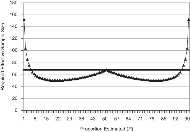
| Final Screening Result Code | Sample Size 2010 |
Sample Size 2011 |
Weighted Percentage 2010 |
Weighted Percentage 2011 |
|---|---|---|---|---|
| NOTE: Some 2010 NSDUH data may differ from previously published data due to updates (see Section B.3 of this report). 1 Examples of “Other, Ineligible” cases are those in which all residents lived in the dwelling unit for less than half of the calendar quarter and dwelling units that were listed in error. 2 “Other, Access Denied” includes all dwelling units to which the field interviewer was denied access, including locked or guarded buildings, gated communities, and other controlled access situations. Source: SAMHSA, Center for Behavioral Health Statistics and Quality, National Survey on Drug Use and Health, 2010 and 2011. |
||||
| TOTAL SAMPLE | 201,865 | 216,521 | 100.00 | 100.00 |
| Ineligible Cases | 35,333 | 37,228 | 17.20 | 16.86 |
| Eligible Cases | 166,532 | 179,293 | 82.80 | 83.14 |
| INELIGIBLES | 35,333 | 37,228 | 17.20 | 16.86 |
| 10 – Vacant | 19,774 | 20,585 | 55.28 | 54.28 |
| 13 – Not a Primary Residence | 8,234 | 8,612 | 24.20 | 24.71 |
| 18 – Not a Dwelling Unit | 2,427 | 2,730 | 6.13 | 6.79 |
| 22 – All Military Personnel | 323 | 370 | 0.88 | 0.96 |
| Other, Ineligible1 | 4,575 | 4,931 | 13.51 | 13.26 |
| ELIGIBLE CASES | 166,532 | 179,293 | 82.80 | 83.14 |
| Screening Complete | 147,010 | 156,048 | 88.42 | 86.98 |
| 30 – No One Selected | 88,085 | 94,342 | 52.50 | 51.82 |
| 31 – One Selected | 32,322 | 34,246 | 19.49 | 19.37 |
| 32 – Two Selected | 26,603 | 27,460 | 16.43 | 15.79 |
| Screening Not Complete | 19,522 | 23,245 | 11.58 | 13.02 |
| 11 – No One Home | 3,111 | 3,124 | 1.79 | 1.71 |
| 12 – Respondent Unavailable | 482 | 579 | 0.28 | 0.32 |
| 14 – Physically or Mentally Incompetent | 423 | 513 | 0.25 | 0.27 |
| 15 – Language Barrier – Hispanic | 65 | 66 | 0.04 | 0.04 |
| 16 – Language Barrier – Other | 504 | 598 | 0.33 | 0.38 |
| 17 – Refusal | 13,034 | 15,589 | 7.82 | 8.72 |
| 21 – Other, Access Denied2 | 1,070 | 2,080 | 0.64 | 1.24 |
| 24 – Other, Eligible | 16 | 13 | 0.01 | 0.01 |
| 27 – Segment Not Accessible | 0 | 0 | 0.00 | 0.00 |
| 33 – Screener Not Returned | 79 | 87 | 0.04 | 0.04 |
| 39 – Fraudulent Case | 736 | 595 | 0.37 | 0.30 |
| 44 – Electronic Screening Problem | 2 | 1 | 0.00 | 0.00 |
| Final Interview Code | 12+ Sample Size 2010 |
12+ Sample Size 2011 |
12+ Weighted Percentage 2010 |
12+ Weighted Percentage 2011 |
12-17 Sample Size 2010 |
12-17 Sample Size 2011 |
12-17 Weighted Percentage 2010 |
12-17 Weighted Percentage 2011 |
18+ Sample Size 2010 |
18+ Sample Size 2011 |
18+ Weighted Percentage 2010 |
18+ Weighted Percentage 2011 |
|---|---|---|---|---|---|---|---|---|---|---|---|---|
| NOTE: Some 2010 NSDUH data may differ from previously published data due to updates (see Section B.3 of this report). 1 “Other” includes eligible person moved, data not received from field, too dangerous to interview, access to building denied, computer problem, and interviewed wrong household member. Source: SAMHSA, Center for Behavioral Health Statistics and Quality, National Survey on Drug Use and Health, 2010 and 2011. |
||||||||||||
| TOTAL | 84,997 | 88,536 | 100.00 | 100.00 | 25,908 | 27,911 | 100.00 | 100.00 | 59,089 | 60,625 | 100.00 | 100.00 |
| 70 – Interview Complete | 67,804 | 70,109 | 74.57 | 74.38 | 21,992 | 23,549 | 84.65 | 84.95 | 45,812 | 46,560 | 73.49 | 73.22 |
| 71 – No One at Dwelling Unit | 1,170 | 1,159 | 1.39 | 1.36 | 202 | 227 | 0.65 | 0.72 | 968 | 932 | 1.47 | 1.43 |
| 72 – Respondent Unavailable | 1,631 | 1,758 | 1.94 | 2.06 | 313 | 337 | 1.22 | 1.19 | 1,318 | 1,421 | 2.02 | 2.16 |
| 73 – Break-Off | 21 | 31 | 0.03 | 0.04 | 4 | 6 | 0.01 | 0.01 | 17 | 25 | 0.04 | 0.05 |
| 74 – Physically/Mentally Incompetent | 877 | 1,003 | 1.81 | 2.01 | 210 | 219 | 0.95 | 0.74 | 667 | 784 | 1.91 | 2.15 |
| 75 – Language Barrier – Hispanic | 126 | 114 | 0.19 | 0.20 | 7 | 7 | 0.03 | 0.03 | 119 | 107 | 0.21 | 0.22 |
| 76 – Language Barrier – Other | 412 | 383 | 1.15 | 1.12 | 20 | 17 | 0.11 | 0.08 | 392 | 366 | 1.26 | 1.24 |
| 77 – Refusal | 9,922 | 10,773 | 17.25 | 17.25 | 756 | 890 | 2.90 | 2.81 | 9,166 | 9,883 | 18.79 | 18.83 |
| 78 – Parental Refusal | 2,286 | 2,538 | 0.87 | 0.89 | 2,286 | 2,538 | 9.01 | 9.02 | 0 | 0 | 0.00 | 0.00 |
| 91 – Fraudulent Case | 21 | 29 | 0.03 | 0.05 | 1 | 7 | 0.00 | 0.05 | 20 | 22 | 0.04 | 0.05 |
| Other1 | 727 | 639 | 0.74 | 0.64 | 117 | 114 | 0.46 | 0.37 | 610 | 525 | 0.78 | 0.66 |
| Demographic Characteristic | Selected Persons 2010 |
Selected Persons 2011 |
Completed Interviews 2010 |
Completed Interviews 2011 |
Weighted Response Rate 2010 |
Weighted Response Rate 2011 |
|---|---|---|---|---|---|---|
| NOTE: Estimates are based on demographic information obtained from screener data and are not consistent with estimates on demographic characteristics presented in the 2010 and 2011 sets of detailed tables. Some 2010 NSDUH data may differ from previously published data due to updates (see Section B.3 of this report). Source: SAMHSA, Center for Behavioral Health Statistics and Quality, National Survey on Drug Use and Health, 2010 and 2011. |
||||||
| TOTAL | 84,997 | 88,536 | 67,804 | 70,109 | 74.57% | 74.38% |
| AGE IN YEARS | ||||||
| 12-17 | 25,908 | 27,911 | 21,992 | 23,549 | 84.65% | 84.95% |
| 18-25 | 28,164 | 28,589 | 23,026 | 23,083 | 81.20% | 80.48% |
| 26 or Older | 30,925 | 32,036 | 22,786 | 23,477 | 72.14% | 71.96% |
| GENDER | ||||||
| Male | 41,782 | 43,436 | 32,826 | 33,779 | 73.11% | 72.49% |
| Female | 43,215 | 45,100 | 34,978 | 36,330 | 75.94% | 76.14% |
| RACE/ETHNICITY | ||||||
| Hispanic | 12,985 | 13,441 | 10,699 | 10,993 | 78.31% | 77.58% |
| White | 55,272 | 57,389 | 43,373 | 44,629 | 73.52% | 73.42% |
| Black | 9,959 | 10,607 | 8,475 | 8,979 | 80.24% | 79.78% |
| All Other Races | 6,781 | 7,099 | 5,257 | 5,508 | 67.11% | 67.74% |
| REGION | ||||||
| Northeast | 16,782 | 17,251 | 13,017 | 13,090 | 72.81% | 69.86% |
| Midwest | 24,139 | 24,570 | 19,301 | 19,258 | 74.81% | 73.92% |
| South | 25,597 | 28,122 | 20,769 | 22,980 | 76.24% | 76.88% |
| West | 18,479 | 18,593 | 14,717 | 14,781 | 73.17% | 74.41% |
| COUNTY TYPE | ||||||
| Large Metropolitan | 38,139 | 38,889 | 29,828 | 30,113 | 73.33% | 72.75% |
| Small Metropolitan | 29,570 | 31,671 | 23,840 | 25,457 | 75.73% | 75.84% |
| Nonmetropolitan | 17,288 | 17,976 | 14,136 | 14,539 | 76.56% | 76.98% |
| Drug/Age Group | 2002 | 2003 | 2004 | 2005 | 2006 | 2007 | 2008 | 2009 | 2010 | 2011 |
|---|---|---|---|---|---|---|---|---|---|---|
| * Low precision; no estimate reported. a Difference between estimate and 2011 estimate is statistically significant at the .05 level. b Difference between estimate and 2011 estimate is statistically significant at the .01 level. Source: SAMHSA, Center for Behavioral Health Statistics and Quality, National Survey on Drug Use and Health, 2002-2011. |
||||||||||
| Marijuana, Aged 26 or Older | 90 | 88 | 176 | 252 | 126 | 134 | 159 | 49b | 247 | 182 |
| Marijuana, Aged 26 to 49 | 90 | 56a | 127 | 122 | 126 | 121 | 155 | 49a | 210 | 138 |
| Any Illicit Drug, Aged 26 or Older | 268 | 324 | 479 | 579 | 415 | 326 | 419 | 433 | 457 | 368 |
| Any Illicit Drug, Aged 26 to 49 | 251 | 209 | 333 | 379 | 405 | 250 | 350 | 205 | 366 | 270 |
| Drug | 2002 | 2003 | 2004 | 2005 | 2006 | 2007 | 2008 | 2009 | 2010 | 2011 |
|---|---|---|---|---|---|---|---|---|---|---|
| * Low precision; no estimate reported. a Difference between estimate and 2011 estimate is statistically significant at the .05 level. b Difference between estimate and 2011 estimate is statistically significant at the .01 level. Source: SAMHSA, Center for Behavioral Health Statistics and Quality, National Survey on Drug Use and Health, 2002-2011. |
||||||||||
| Marijuana | 31.2 | 29.6 | 29.5 | 30.4 | 29.1 | 32.4 | 32.6 | 32.2 | 36.3a | 29.5 |
| Any Illicit Drug | 34.8 | 32.8 | 31.6 | 34.0 | 33.9 | 32.9 | 35.1 | 31.7 | 37.2 | 33.0 |
| Domains | 2010 Population Based on 2000 Census |
2010 Population Based on 2010 Census |
Difference in 2010 Population Based on 2010 Census versus 2000 Census1 |
Percent Difference Relative to 2010 Population Based on 2000 Census2 |
|---|---|---|---|---|
| NOTE: Population counts are annualized estimates of the 2010 population and reflect the population of the entire year. 1 Difference between the number of people in the 2010 population overall or in a given subgroup from control totals based on the 2010 census and the corresponding number from control totals based on the 2000 census. 2 Based on the following formula: {[(2010 Population Based on 2010 Census) − (2010 Population Based on 2000 Census)] ÷ (2010 Population Based on 2000 Census)} × 100. 3 Unlike racial/ethnic groups discussed elsewhere in this report, race domains in this table include Hispanics in addition to persons who were not Hispanic. Source: SAMHSA, Center for Behavioral Health Statistics and Quality, National Survey on Drug Use and Health, 2010. |
||||
| TOTAL | 253,619,107 | 255,331,811 | 1,712,704 | 0.68% |
| 12 to 17 | 24,346,528 | 25,156,348 | 809,820 | 3.33% |
| 18 to 25 | 34,072,349 | 34,010,012 | −62,338 | −0.18% |
| 26 to 34 | 36,523,574 | 35,840,157 | −683,416 | −1.87% |
| 35 to 49 | 62,042,733 | 62,422,429 | 379,696 | 0.61% |
| 50-64 | 57,695,892 | 58,701,774 | 1,005,882 | 1.74% |
| 65 or Older | 38,938,030 | 39,201,090 | 263,060 | 0.68% |
| Male | 123,430,407 | 123,422,261 | −8,146 | −0.01% |
| Female | 130,188,700 | 131,909,550 | 1,720,850 | 1.32% |
| Hispanic | 36,769,252 | 38,346,951 | 1,577,700 | 4.29% |
| Not Hispanic | 216,849,855 | 216,984,859 | 135,004 | 0.06% |
| White3 | 204,032,161 | 202,851,643 | −1,180,518 | −0.58% |
| Black3 | 31,168,385 | 31,618,096 | 449,711 | 1.44% |
| American Indian or Alaska Native3 | 2,483,390 | 2,905,990 | 422,600 | 17.02% |
| Asian3 | 11,915,744 | 12,869,433 | 953,689 | 8.00% |
| Native Hawaiian or Other Pacific Islander3 | 460,327 | 527,384 | 67,057 | 14.57% |
| Two or More Races3 | 3,559,100 | 4,559,265 | 1,000,165 | 28.10% |
| 2011 versus 2010 (New) Estimated Numbers, Significant |
2011 versus 2010 (New) Estimated Numbers, Not Significant |
2011 versus 2010 (New) Estimated Percentages, Significant |
2011 versus 2010 (New) Estimated Percentages, Not Significant |
2011 versus 2010 (New) Mean Age At First Use, Significant |
2011 versus 2010 (New) Mean Age At First Use, Not Significant |
|
|---|---|---|---|---|---|---|
| 2010 (Old) = Estimates for 2010 with weights poststratified to 2010 control totals based on the 2000 census; 2010 (New) = Estimates for 2010 with weights poststratified to 2010 control totals based on the 2010 census. NOTE: There are 26 tests not included due to suppression, 13 each for totals and percentages. Tests were conducted at the .05 level of significance. Cells with bolded data indicate consistent outcomes between 2011 versus 2010 (New) and between 2011 versus 2010 (Old). Source: SAMHSA, Center for Behavioral Health Statistics and Quality, National Survey on Drug Use and Health, 2010 and 2011. |
||||||
| 2011 versus 2010 (Old), Significant |
33 | 30 | 45 | 19 | 0 | 0 |
| 2011 versus 2010 (Old), Not Significant |
6 | 432 | 0 | 371 | 0 | 66 |
| 2011 < 2010 (New), Number (Percent) |
No Difference between 2011 and 2010 (New) Number (Percent) |
2011 > 2010 (New), Number (Percent) |
|
|---|---|---|---|
| 2010 (Old) = Estimates for 2010 with weights poststratified to 2010 control totals based on the 2000 census; 2010 (New) = Estimates for 2010 with weights poststratified to 2010 control totals based on the 2010 census. NOTE: Significance testing is based on a 2-sided test at the 0.05 level of significance. Cells with bolded data indicate consistent outcomes between 2011 versus 2010 (New) and between 2011 versus 2010 (Old). Source: SAMHSA, Center for Behavioral Health Statistics and Quality, National Survey on Drug Use and Health, 2010 and 2011. |
|||
| 2011 < 2010 (Old) | 67 (6.7%) | 32 (3.2%) | 0 (0.0%) |
| No Difference between 2011 and 2010 (Old) | 5 (0.5%) | 869 (86.7%) | 1 (0.1%) |
| 2011 > 2010 (Old) | 0 (0.0%) | 17 (1.7%) | 11 (1.1%) |





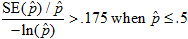
 > .175
 , or
, or > .175
 , or
, or
 .
. .
.